








Blog
Replacing a Fuel Cell Circuit with Machine Learning Metamodels: Up to 7x faster vehicle simulation with the Machine Learning Assistant in GT-SUITE
Overview
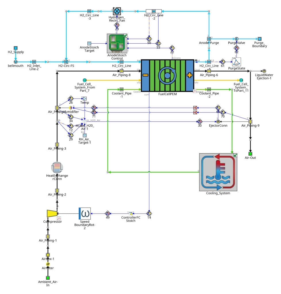
Fuel cell vehicle models are rich in physics and relatively fast to simulate, but when running many drive-cycle or duty-cycle simulations, for example for controls development, more speed is always desired. The flow circuit and cooling system are often the heaviest part of an integrated vehicle simulation. If you only need the stack’s main outputs for a drive-cycle, do you need to solve all that physics every time?
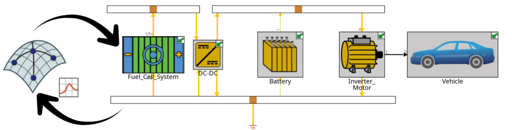
We tested this with the Machine Learning Assistant (MLA) in GT-SUITE. We replaced the fuel cell flow circuit and cooling system with metamodels. In this post, we cover the approach, the lessons learned, and the speed-ups.
The goal
We started from the Fuel_Cell_Vehicle-Flow.gtm example model (available within GT-SUITE). The aim was to swap out the fuel cell circuit and its cooling system with metamodels, without changing the rest of the vehicle. The metamodels had to predict four responses:
- Stack voltage
- Stack temperature
- MWC
- Compressor power
The main available input was the current coming from the DC converter.
Step 1: Getting the right training data
For dynamic regression metamodels on drive-cycle simulations, we’ve seen in other engineering domains that artificially designed simulations can give poor predictions on realistic drive cycles. The likely reason is that designed inputs don’t have the same dynamics as real drive cycles. It works in some domains but not all. For this project, several designed-simulation approaches were tried and didn’t work.
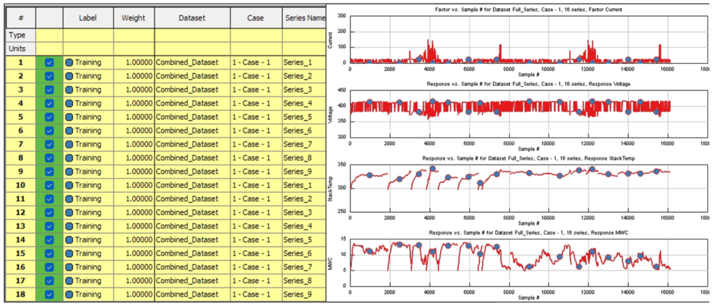
So we trained on drive cycles instead. The example model had 4 drive-cycle cases. Looking at the data in the MLA showed we needed more variation, especially in MWC. We did two things:
- Added 5 more drive cycles to the model.
- Copied the model and initialized the cases at a higher temperature, giving ColdStarts and WarmStarts
Combining the two gave a single dataset of 18 drive-cycle series.
Step 2: Splitting data into training, validation, and test sets
Why we didn’t use the default split
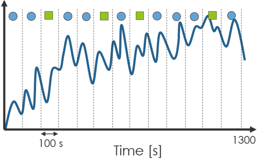
For drive-cycle data, we’ve found an alternative works much better to labeling entire series as training, validation, or test:
- Pick 2–3 series for testing.
- Cut all other series into 100-second segments. The MLA’s segmentation button on the Select Series page does this.
- Randomly split those segments 75% training and 25% validation.
Step 3: The modeling approach
We used a combination of static and dynamic regression metamodels to accurately predict the voltage, stack temperature, MWC, and compressor power using the current as the sole input.
Results
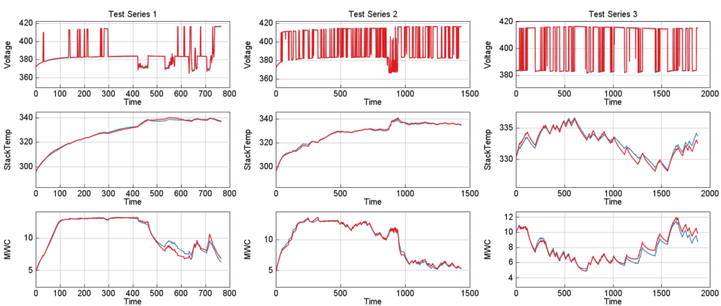
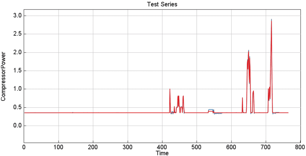
The comparison between the simulation dataset and metamodel prediction is carried out on the graph below for the time series not used during the training and considered as “test” series. As we can see the metamodel correlates very well with the ground truth indicating that it generalizes well to those unseen data.
Putting it in the vehicle model
The metamodels are exported as .mmp files and brought into the vehicle model with the MetamodelHarness template. Then:
- The fuel cell flow circuit and its cooling system are removed.
- The NARX voltage prediction drives a new part based on the SourceVoltage
- Run Setup > SignalControl evaluates the metamodels at a 1-second time step.
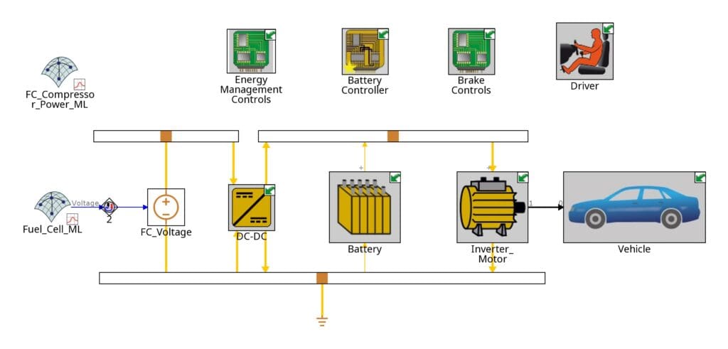
Two settings are worth knowing about:
- Initial output values: NARX initial outputs matter for every simulation. A “Duration at Initial Output” of 1 second avoided unrealistic predictions that otherwise persisted for the first 20 seconds.
- Actuation delay: Because the prediction is imposed on the SourceVoltage by actuation, voltage has a 1-second delay. It doesn’t noticeably affect the overall results.
We also checked that battery state of charge and electric motor power were essentially unchanged, so the rest of the powertrain behaves the same.
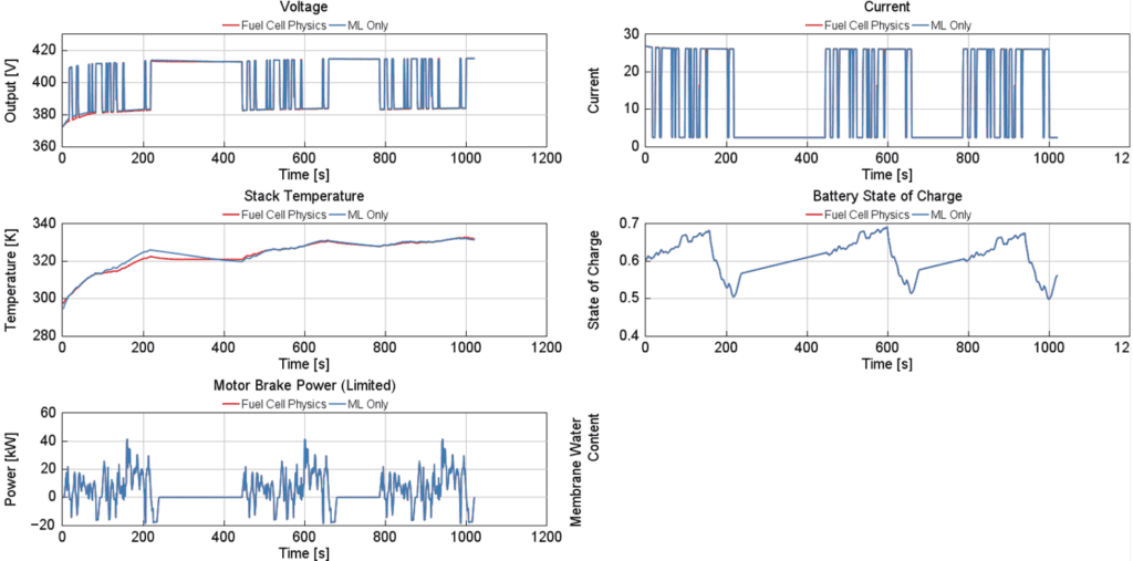
The payoff: faster simulations
Across nine drive-cycle cases, the ML-only model ran 1.6x to 7.0x faster than the full fuel cell physics model, roughly 3x on average.
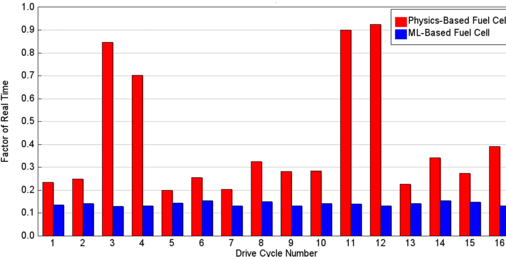
What this means for fuel cell vehicle teams
This case study shows that machine learning can be a practical way to speed up fuel cell vehicle simulation. By replacing the fuel cell flow circuit and cooling system with metamodels built in the Machine Learning Assistant, the integrated vehicle model ran between 1.6x and 7.0x faster across nine drive-cycle cases, roughly 3x on average. The rest of the powertrain, including battery state of charge and electric motor power, was essentially unchanged.
The benefits go beyond raw speed:
- Faster iteration. Shorter run times mean more drive cycles, more design variants, and more what-if studies in the same amount of time.
- Fidelity where it matters. Only the fuel cell circuit is replaced. The vehicle, battery, and electric drive stay fully physics-based, so the system-level picture is preserved.
- A compact, reusable model. The metamodels are exported as .mmp files and dropped into the vehicle model with the MetamodelHarness template, using current as the only input.
- Quick to build. Each metamodel trains quickly, so engineers can run grid searches over many configurations and pick the best one using validation error.
With a sound data strategy (realistic drive cycles, enough variation, and a thoughtful training, validation, and test split), metamodels become a dependable complement to physics-based models. For teams working on fuel cell powertrains, that means getting answers sooner, and exploring more of the design space, without leaving GT-SUITE.
See how the Machine Learning Assistant in GT-SUITE can turn slow physics subsystems into fast, accurate metamodels. To learn more about how GT-SUITE can help you model and develop fuel cell systems, please visit our webpage on the topic: Fuel Cell System Modeling, or contact us! Follow our LinkedIn channel to stay updated on the latest advancements in our solutions and subscribe to the GT blog to receive updates on new AI capabilities, engineering solutions, and industry trends.
Frequently asked question
1. What is the Machine Learning Assistant (MLA) in GT-SUITE?
The MLA is a GT-SUITE tool for building machine learning metamodels from simulation data. In this case study, it was used to replace the fuel cell flow circuit and cooling system with fast metamodels that predict stack voltage, stack temperature, MWC, and compressor power.
2. How much faster is the vehicle simulation with metamodels?
Across nine drive-cycle cases, the ML-based model ran 1.6x to 7.0x faster than the full physics model, roughly 3x on average. Battery state of charge and electric motor power stayed essentially unchanged.
3. What training data do I need for accurate drive-cycle metamodels?
Realistic drive cycles with enough variation. Here, 18 drive-cycle series were used (including cold-start and warm-start versions), with 2-3 series held out for testing. The remaining series were cut into 100-second segments and split 75% training and 25% validation.